
The concept
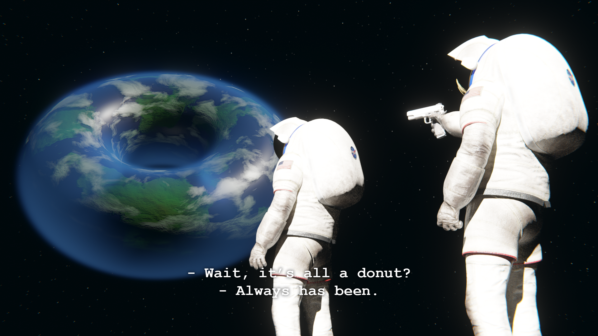
Lets start with a medium level concept, then we will inspect a harder one, so we can understand the last part easily. This is a Clifford torus, drawn by Sirius—A:
In geometric topology, it is the simplest and most symmetric flat embedding of the Cartesian product of two circles \(\color{#217ABE}{S^1_a}\) and \(\color{#217ABE}{S^1_b}\) (in the same sense that the surface of a cylinder is “flat”). It is named after William Kingdon Clifford.
A normal torus is basically a a tube shape that looks like a doughnut or an inner tube, created by revolving a circle in the \(\color{#217ABE}{\rm 3rd}\) dimension around a circle, which is why a torus is a “surface of revolution.
Here is a link to a Desmos page of the graph above, go ahead, play with it. When you change the \(\color{#217ABE}{\rm 3D}\) properties (\(\color{#217ABE}{X}\), \(\color{#217ABE}{Y}\) and \(\color{#217ABE}{Z}\)), you can just see the doughnut rotating.
But when you play with the \(\color{#217ABE}{\rm 4th}\) dimension (\(\color{#217ABE}{W}\)), your doughnut seems to lose its \(\color{#217ABE}{\rm 3D}\) form, meaning, you can’t \(\color{#217ABE}{imagine}\) what’s going on physically. Or, in a sense, your doughnut was a \(\color{#217ABE}{\rm 4D}\) object and you could only understand it \(\color{#217ABE}{\rm 3D}\) ly.
Cosmos: Neil’s 2D Civilization
However, before playing more with the Clifford Torus, I suggest reading the rest of this post. And before that, I strongly suggest watching Neil deGrasse Tyson explaining a \(\color{#217ABE}{\rm 2D}\) civilization here:
When he mouth-dubs the \(\color{#217ABE}{\rm 2D}\) alien with a squeaky voice, try not to laugh too loud.
The Clifford torus at the top of this post, is made with Desmos 2D by its author, probably when there was no Desmos 3D around and migrating it is unnecessary for this post for now. If you want to examine a \(\color{#217ABE}{\rm 2D}\) point of view, I prepared another example with Desmos 3D:
Imagine the Neil’s little alien living in the \(\color{#217ABE}{XY}\) plane of tihs graph. Our cube is just a regular hexagon for him. When a \(\color{#217ABE}{\rm 3D}\) being manipulates the cube (you, rotating it), the little guy doesn’t understand what’s going on. The hexagon just turned into a rectangle!
Freefall
In our universe, it is clear that mathematical rules are present. We will analyse an example of a ball falling down, for the young philosophers which may say;
Math isn’t real. Humanity invented it.
When my highschool philosophy teacher told us this, I saw an opportunity to disrupt the class (it was kind of my duty, expected of me from my classmates) and talked about it till the class is dismissed, but the time wasn’t enough, and I was young and dumb enough, so wasn’t able to persuade him to see that Math is the universal truth.
Young me would say, “An apple was falling down from the tree the same way before Sir Isaac Newton discovered gravity.” or “Newton’s discoveries, didn’t alter the trajectory of a poor man’s head as it fell to the ground, separated from his body by a sudden sword strike.” but present-me will explain it to you.
When a stone falls toward Earth, its height decreases as it accelerates, governed by the equation: the product of Earth’s gravitational acceleration and the square of time, divided by two. More clearly, the distance \(\color{#217ABE}{d}\) travelled by an object falling for time \(\color{#217ABE}{t}\):
\[ d = \frac{g·t^2}{\rm 2} \]
Air friction or another force of attraction can be ‘included’ in the calculation, but these additions complicate the formula and increase its precision, without invalidating the basic calculation. Below, you can find a kind of a \(\color{#217ABE}{20}\ {\rm fps}\) recording of a ball falling:
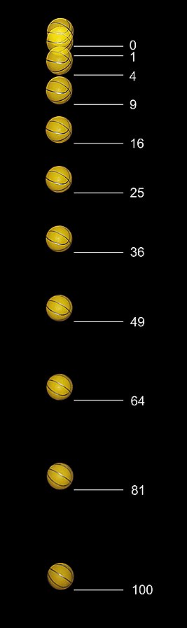
The numbers represent positions. An initially-stationary object (the basketball) which is allowed to fall freely under gravity, drops a distance which is proportional to the square of the elapsed time. The original image, spanning half a second, was captured with a stroboscopic flash at \(\color{#217ABE}{\rm 20}\) flashes per second and showing the positions till \(\color{#217ABE}{100}\) . I clipped it to \(\color{#217ABE}{36}\) to invade less space in the post.
During the first \(\color{#217ABE}{1/20th}\) of a second the ball drops \(\color{#217ABE}{1}\) unit of distance (here, a unit is about 12 mm), by \(\color{#217ABE}{2/20th}\)s, it has dropped at total of \(\color{#217ABE}{4}\) units, by \(\color{#217ABE}{3/20th}\)s, \(\color{#217ABE}{9}\) units and so on.
Even though this image wasn’t recorded in a vacuum, the observation matches with the formula because the timeframe is just half a second. If it was longer, the result would start being quite inaccurate after only \(\color{#217ABE}{\rm 5}\) seconds of fall, at which time an object’s velocity will be a little less than the vacuum value of
\[ 9.8\ \color{#428400}{\mathrm{m/s^{2}}} × 5\ \color{#428400}{\mathrm{s}} = 49\ \color{#428400}{\mathrm{m/s}} \]
due to air resistance.
While trying to make you see that the math behind the freefall is accurate, you may come to see the inaccuracies induced by air friction. Then watch this video that was recorded in the NASA’s Space Power Facility in Ohio to see how freefalling objects behave in a very expensive, huge, airless space:
Do you still have questions? Are you really going to joke about time being relative? I would answer:
It’s not that relative bro.
Meaning, with the speeds we use in our freefall operations, relativeness of time is insignificant, microscopic, miniature.
How about the definition of a second, a meter, or the gravity constant? Aren’t we just defining them?
Would changing these constants or definitions change the reality? The formula? \(\color{#217ABE}{No}\).
\[ d = \frac{g·t^2}{\rm 2} \]
is, still the truth.
How? Let’s dive.
The planck constant and E = h·f
We historically defined the second as \(\color{#217ABE}{1⁄86\ 400}\) of an earth day. Now we define it as Caesium-133’s fixed unperturbed ground-state hyperfine transition frequency, denoted by \(\color{#217ABE}{Δν_{\rm Cs}}\) which is \(\color{#217ABE}{9\ 192\ 631\ 770}\ \color{#428400}{\rm Hz}\) as we realised that it is pretty stable. Basically it ticks approximately every \(\color{#217ABE}{\rm 9}\) trillionth of a second:
\[ 1\ {\rm s} = \frac{9\ 192\ 631\ 770}{Δν_{\rm Cs}}\ ⇔\ 1\ {\rm Hz} = \frac{Δν_{\rm Cs}}{9\ 192\ 631\ 770} \]
A meter is also a definition but since 2019, the metre has been defined as the length of the path travelled by light in vacuum during a time interval of \(\color{#217ABE}{1/299\ 792\ 458th}\) of a second, so the definition of a meter would be:
\[ c = 299\ 792\ 458\ \mathrm {\color{#428400}{m/s}} \]
\[ 1\ {\rm m} = \frac{9\ 192\ 631\ 770}{299\ 792\ 458} \color{#428400}{\frac{c}{Δν_{\rm Cs}}} ≈ 30.6633189884983\ \color{#428400}{\frac{c}{Δν_{\rm Cs}}} \]
Earth’s gravity, denoted by \(\color{#217ABE}{\bf g}\), agreed upon as \(\color{#217ABE}{9.80665}\ \color{#428400}{\rm m/s^2}\), even though we see it as a constant, is also a definition. It slightly varies according to where you are at, from approximately \(\color{#217ABE}{9.78}\ \mathrm {\color{#428400}{m/s^2}}\) at the Equator to approximately \(\color{#217ABE}{9.83}\ \mathrm {\color{#428400}{m/s^2}}\) at the poles.
Here comes the fun part… If you are a fan of Fermi paradox, imagine long-extinct interstellar ancestors of us, who lived in another galaxy before eventually reaching Earth.
But if you’re a fun person, consider the idea of a theoretical alien civilization in a distant galaxy that emerged and developed in ways remarkably similar to our own. Let’s name these guys “Vortigaunts” like the game \(\color{#23a493}{\enclose{circle}{\lambda}}\) Half-Life does, so we may calculate their \(\color{#217ABE}{G_{\rm \color{#23a493}{vort}}}\) value.

Their day length is most probably different, their distance unit is different. If they develop a space travel and visit Earth, and do decide to do some math since their ship needs a smooth landing, the value of the \(\color{#217ABE}{g_{\color{#1d4ed8}{earth}}}\) constant would be a different value for their calculation. How?
\(\color{#217ABE}{G}\), the universal gravitational constant was measured by Newton, via observing celestial objects. Or you can call it \(\color{#217ABE}{G_{\rm \color{#1d4ed8}{Earthling}}}\) for being specific but since Earthlings are going to read this post;
\[ G = 6.6743×10^{−11} \ \mathrm{\color{#428400}{\frac{m^{3}}{kg·s^2}}} \]
\[ {\rm kg} ≈ 1.475521399 × 10^{40}\ \color{#428400}{\frac{h·Δν_{\rm Cs}}{c^2}} \]
We have already defined \(\color{#217ABE}{Δν_{\rm Cs}}\) above. The \(\color{#217ABE}{h}\) in the definition of the unit \(\color{#217ABE}{\rm kg}\) above, is the planck constant, also measured by universal observations, by Max Planck:
\[ h = 6.62607015×10^{−34}\ \color{#428400}{\rm{\frac{kg·m^2}{s}}} \]
As you can see, the unit of the planck constant has a kilogram and the unit of the kilogram has a planck constant in it!
Well, this doesn’t mean that planck constant isn’t real. We just didn’t know it when French defined what a kilogram was.
Originally, The kilogram used to be defined by a physical object (the Le Grand K in France). Its mass could change due to wear, contamination, or environmental factors. By linking the kilogram to \(\color{#217ABE}{h}\) through quantum mechanics and the equation \(\color{#217ABE}{E=h·f}\), we tied the unit of mass to a fixed value of energy. This makes the kilogram independent of any physical object.
The value of \(\color{#217ABE}{h}\) was experimentally measured before the redefinition using precise experiments like the Kibble balance and Avogadro project. These experiments linked \(\color{#217ABE}{h}\) to the old kilogram definition.
Once \(\color{#217ABE}{h}\) was determined with incredible accuracy, the kilogram was redefined in terms of \(\color{#217ABE}{h}\). Now, \(\color{#217ABE}{h}\) has a fixed value:
\[ h = 6.62607015×10^{−34}\ \color{#428400}{\rm kg·m^2·s^{-1}} \]
If you strip away all the human-defined units —\(\color{#217ABE}{\rm kg}\), \(\color{#217ABE}{\rm m}\), \(\color{#217ABE}{\rm s}\)— and express the universe in its natural language, the planck constant and the relationship it defines; \(\color{#217ABE}{E=h·f}\) still holds. Energy and frequency are linked by the same proportionality, no matter where you are in the cosmos:
\[ E=h·f \]
Does that mean the value of \(\color{#217ABE}{G}\) is universal? Yes & No… If you use \(\color{#217ABE}{\rm kg}\), \(\color{#217ABE}{\rm m}\), \(\color{#217ABE}{\rm s}\) in your other equations, Yes! But if you don’t, No.
Check the observable effects of \(\color{#217ABE}{E=h·f}\) on Earth 🌍, and and outside 🪐 below and you will find out why \(\color{#217ABE}{\rm kg}\), \(\color{#217ABE}{\rm m}\), \(\color{#217ABE}{\rm s}\) doesn’t matter and why we have defined them with the universal constants like planck constant and light speed.
🌐 Observable effects of E=h·f on Earth
-
Ultraviolet (UV) light has shorter wavelengths (higher \(\color{#217ABE}{f}\), so higher energy) than visible light. This is why UV light can cause sunburns, while visible light doesn’t.
-
When you are out at night, watching stars with your telescope, using red light allows you to preserve your dark adaptation. Because red light is dim and carries less energy (less \(\color{#217ABE}{f}\) ), so it’s less disruptive to rod cells. The human eye adjusts to darkness using rod cells (sensitive to dim light) and cone cells (sensitive to color). Bright blue or white light(which has a blue component) can quickly reset the rod cells, ruining night vision.
-
You may have used pocket solar panels to charge your phone while camping or bigger ones to supply electrical energy to your house. What is happening behind the scenes? Photons from sunlight hit semiconductors in your solar panel, and if the energy ( \(\color{#217ABE}{h⋅f}\) ) is enough to free electrons, those semiconductors generate electric current.
-
In radio communication, electrons oscillate in an antenna at a specific frequency, emitting electromagnetic waves with energy: \(\color{#217ABE}{E=h⋅f}\). The low frequencies of radio waves correspond to lower energies, making them ideal for long-distance communication. Because this energy is so small, they are ideal for transmitting signals with minimal power loss and no damage to biological tissue.
🪐 Observable effects of E=h·f outside
-
Gamma Rays from supernovae are another perfect example. These rays are extremely high-frequency, carrying tons of energy, and this demonstrates how frequency directly translates into energy, just like the formula \(\color{#217ABE}{E=h⋅f}\) predicts. Charles Meegan of NASA’s Marshall Space Flight Center said “Gamma-ray bursts are so bright we can see them from billions of light-years away, which means they occurred billions of years ago, and we see them as they looked then”.
-
X-rays are high-energy radiation emitted by celestial bodies. Astronomers can observe X-rays coming from objects like black holes or neutron stars. These X-rays have a much higher frequency ( \(\color{#217ABE}{f}\) ) than visible light, so they carry much more energy. This is why X-rays can be harmful and why spacecraft use shielding to protect sensitive equipment.
The universal gravitational costant
Let’s go back to the \(\color{#217ABE}{G}\). Now we established that the planck constant, even though its unit includes a human defined construct like a kilogram \(\color{#217ABE}{\rm kg}\) or a second \(\color{#217ABE}{\rm s}\), its presence in the universe is proven. Now we can see how the earth’s gravity is calculated by Earthlings.
But instead of using variables like \(\color{#217ABE}{g_{Earth_{earthling}}}\) and \(\color{#217ABE}{g_{Earth_{vortigaunt}}}\), we will use colors and symbols to simplify the formulae.
\[ \color{#217ABE}{g}_ \color{#1d4ed8}{\rm 🜨} \]
for our gravity, calculated by we Earthlings
\[ \color{#217ABE}{g}_{\rm \color{#23a493}{🜨_V}} \]
is what Vortigaunts can use with their units
Because the earth is \(\color{#1d4ed8}{Blue}\) and I assume the Vortagron is \(\color{#23a493}{Jungle\ Green}\). Also showing these colors for units will further simplify the formulae.
This is how we Earthlings calculate the gravity of Earth:
\[ g_{\rm \color{#1d4ed8}{🜨}} = \frac{G_{\rm {\color{#1d4ed8}{m}^3· \color{#1d4ed8}{kg}^{-1} \color{#1d4ed8}{s}^{{-2}}}}×M_{\rm \color{#1d4ed8}{kg}}}{R^2_{\rm \color{#1d4ed8}{{m}}}} = 9.82030229339\ \color{#1d4ed8}{\rm m}/\color{#1d4ed8}{\rm s}^2 \]
Here, the value of \(\color{#217ABE}{G}\) is:
\[ G_{\rm \color{#1d4ed8}{Earthling}} = 6.6743×10^{-11}\ \rm \color{#1d4ed8}{m}^3⋅\color{#1d4ed8}{kg}^{-1}⋅\color{#1d4ed8}{s}^{-2} \]
The meter was originally defined in 1791 by the French National Assembly as one ten-millionth of the distance from the equator to the North Pole along a great circle (with a little error but that’s not important for us since it is just a definition), so the Earth’s polar circumference is approximately 40000 km.
The kilogram, although defined with the planck constant now, was defined in a similar way (with a reference: a mass equal to the mass of \(\rm \color{#217ABE}{1\ dm^3}\)) of water at the temperature of its maximum density, which is at approximately \(\rm \color{#217ABE}{+4 }\) °C, it is tied to a volume, which is a universal 3D thing through meter definition.
The second is also similar, with a reference to \(\color{#217ABE}{1/86400}\) of an Earth day like we mentioned above.
Vortigaunt units
Let’s redefine the kilogram (\(\color{#217ABE}{\rm kg}\)), meter (\(\color{#217ABE}{\rm m}\)) and second (\(\color{#217ABE}{\rm s}\))!

Let’s suppose French Vortigaunts from the planet Vortagron, defined the meter, kilogram and second, based on their planet; They have a giant fruit called Vorfruit, with a very standard size and weight roughly \(\color{#217ABE}{0.333}\) of an Earthling meter and \(\color{#217ABE}{0.5}\) Earthling kilograms.
I am re-thinking of the Vortigaunts of the game \(\color{#23a493}{\enclose{circle}{\lambda}}\) Half-Life for the argument’s sake and making their perception of time \(\color{#217ABE}{2}\) times faster than ours, by a nice inspiration from the game’s name. Since they are the ones that are visiting Earth in this simulation, and not us visiting Vortagron, their civilization should have developed faster than us. To summarize;
\(\color{#217ABE}{3}\) vorlen ≈ \(\color{#217ABE}{1}\) meter
\(\color{#217ABE}{2}\) vormas ≈ \(\color{#217ABE}{1}\) kilogram
\(\color{#217ABE}{2}\) vorsec ≈ \(\color{#217ABE}{1}\) second
They could have developed an atomic clock and more standardised stuff like our caesium standard, but they would still have these units, just like us. I gave these just for reference since we decided to use colors to simplify the formulae:
\[ \color{#1d4ed8}{\rm m} = 3\ \color{#23a493}{\rm m_v} \]
\[ \color{#1d4ed8}{\rm kg} = 2\ \color{#23a493}{\rm kg_v} \]
\[ \color{#1d4ed8}{\rm s} = 2\ \color{#23a493}{\rm s_v} \]
Our value for the \(\color{#217ABE}{G}\) was:
\[ G_{\rm \color{#1d4ed8}{Earthling}} = 6.6743(15)×10^{-11}\ \rm \color{#1d4ed8}{m}^3⋅\color{#1d4ed8}{kg}^{-1}⋅\color{#1d4ed8}{s}^{-2} \]
So with the Vortigaunt units;
\[ G_{\rm \color{#23a493}{Vortigaunt}} = G_{\rm \color{#1d4ed8}{Earthling}}×\frac{27}{8}\ \rm \color{#23a493}{m_v}^3⋅\color{#23a493}{kg_v}^{-1}⋅\color{#23a493}{s_v}^{-2} \]
\[ G_{\rm \color{#23a493}{Vortigaunt}} = G_{\rm \color{#23a493}{V}} = 2.25257625×10^{-10}\ \rm \color{#23a493}{m_v}^3⋅\color{#23a493}{kg_v}^{-1}⋅\color{#23a493}{s_v}^{-2} \]
Let’s go for their gravity of Earth calculation:
\[ g_{\rm \color{#23a493}{🜨_V}} = \frac{G_{\rm \color{#23a493}{V}} ⋅ M_{\rm \color{#23a493}{🜨v}}}{R_{\rm \color{#23a493}{🜨_V}}^2} \]
\[ M_{\rm \color{#1d4ed8}{🜨}} = 5.9722×10^{24}\ \color{#1d4ed8}{\rm kg}\ ⇒\ M_{\rm \color{#23a493}{🜨_V}} = 2⋅M_{\rm \color{#1d4ed8}{🜨}} = 1.19444×10^{25}\ \color{#23a493}{\rm kg_v} \]
\[ R_{\rm \color{#1d4ed8}{🜨}} = 6371000\ \color{#1d4ed8}{\rm m}\ ⇒\ 3 ⋅ R_{\rm \color{#1d4ed8}{🜨}} = R_{\rm \color{#23a493}{🜨_V}} = 19113000\ \color{#23a493}{\rm m_v} \]
Now we can calculate the Earth’s gravity in Vortigaunt units:
\[ g_{\rm \color{#23a493}{🜨_V}} = \frac{2.25257625×10^{-10} ⋅ 1.19444×10^{25}}{19113000^2} = 7.36522672004\ \color{#23a493}{\rm m_v}/\color{#23a493}{\rm s_v}^2 \]
Okay… what can we do with this value? We can do Vortigaunt physics! Remember the distance traveled formula for a freefall:
\[ d = \frac{g·t^2}{\rm 2} \]
If we were using a non stationary object, we would use \(\color{#217ABE}{v_0 t + \frac{1}{2} gt^2}\). To simplify, we are using the stationary formula above. So let’s say a stationary object falls for \(\color{#217ABE}{2}\) seconds, the traveled distance would be:
\[ d_{\rm \color{#1d4ed8}{ m}} = \frac{g_{\rm \color{#1d4ed8}{🜨}}·t_{\rm \color{#1d4ed8}{\rm s}}^2}{\rm 2} = \frac{9.82030229339·2^2}{2} = 19.6406045868\ {\rm \color{#1d4ed8}{ m}} \]
Let’s try it with the Vortigaunt math. If it produces the same result, we can say that this formula is a universal truth!
Our \(\color{#217ABE}{2}\) seconds(\({\rm \color{#1d4ed8}{\rm s}}\)) is \(\color{#217ABE}{4}\) vorsecs(\({\rm \color{#23a493}{\rm s}}\)), and we have calculated the value of \(\color{#217ABE}{g}_{\rm \color{#23a493}{🜨_V}}\) so:
\[ d_{\color{#23a493}{\rm v}} = \frac{g_{\rm \color{#23a493}{🜨_V}}·t_{\color{#23a493}{\rm v}}^2}{\rm 2} = \frac{7.36522672004·4^2}{2} = 58.9218137603 \ \color{#23a493}{\rm m_v} \]
Look at the result. Isn’t it \(\rm \it \color{#217ABE}{beautiful}\) ?
\[ \rm 58.9218137603\ \color{#23a493}{m_v} = 19.6406045868\ \color{#1d4ed8}{m} \]
That’s why, we redefined the SI units with universal constants.
Well, you can say;
Arithmetics don’t exist. We made it up.
I’d say then if numbers are not real, give me half of your gold coins 🪙 To win the the argument, if you are generous enough, you would do it. Let me tell you something you cannot do. You can’t give me 1.5 times what you have.
No matter how much coins 🪙 you have, if you try to give me 1.5 times (or 2) times of it, since your current amount of coins 🪙 is changed, ∴ the amount of “1.5 times what you have” changes. If you are trying to win the argument by zero coins, watch this video. Zero doesn’t exist:
E = m·c²
Nice subtitle isn’t it? Don’t worry, If you focus, the concept is easy to grasp.
This part is just an extra or an easter egg for those who wonder the relation between \(\color{#217ABE}{E=h⋅f}\) and Einstein’s famous equation, \(\color{#217ABE}{E=m⋅c^2}\). Most of us don’t know its full form:
\[ E_\text{rel} = \sqrt{(m_{0}⋅c^2)^2+p^2⋅c^2} \]
For photons, where \(\color{#217ABE}{m_{0} = 0}\), the equation becomes:
\[ E_{\text{rel}} = p \cdot c \]
Here, \(\color{#217ABE}{p}\) is the momentum of the photon. But how does this relate to \(\color{#217ABE}{E=h⋅f}\)?
Photons have momentum, even though they have no rest mass. Their momentum \(p\) is given by:
\[ p = \frac{h}{\lambda} \]
where \(\color{#217ABE}{h}\) is Planck’s constant and \(\color{#217ABE}{\lambda}\) is the wavelength of the photon. Using the relationship between frequency and wavelength \(\color{#217ABE}{f = \frac{c}{\lambda}}\), we can rewrite momentum as:
\[ p = \frac{h \cdot f}{c} \]
Substitute this into the relativistic energy equation \(\color{#217ABE}{E_{\text{rel}} = p \cdot c}\):
\[ E_{\text{rel}} = \left(\frac{h \cdot f}{c}\right) \cdot c = h \cdot f \]
This shows that for photons, Einstein’s relativistic energy formula \(\color{#217ABE}{E_{\text{rel}} = p \cdot c}\) naturally leads to Planck’s relation \(\color{#217ABE}{E = h \cdot f}\).
In other words, the energy of a photon as described by Einstein’s relativity is entirely consistent with the quantum description of energy in terms of frequency. Both equations describe the same physical reality for photons, just from slightly different perspectives.
The Conjecture
Finally, since we established that math is, in fact; real, not a human construct but a universal rule, we can go back to the main topic. We can first prove the third dimension that we live in, within the second dimension.
Let’s show a 2D point \(\color{#217ABE}{{\rm P_{0}} = (x_0,y_0)}\) like this:
\[ {\rm P_{0}} = \left\lbrack\ \matrix { x_0 \cr y_0 } \ \right\rbrack \]
To do a \(\color{#217ABE}{θ}\) degrees of rotation, you can use a rotation matrix \(\color{#217ABE}{\rm R}\), the middle matrix below:
\[ \rm P_1 = R·P_0 \]
\[ \left\lbrack\ \matrix { x_1 \cr y_1 } \ \right\rbrack = \left\lbrack\ \matrix { cos(θ) & -sin(θ) \cr sin(θ) & cos(θ) } \ \right\rbrack \left\lbrack\ \matrix { x_0 \cr y_0 } \ \right\rbrack \]
Then, translation of this point is also simple if you translate \(\color{#217ABE}{x_1}\) by \(\color{#217ABE}{a}\) and \(\color{#217ABE}{y_1}\) by \(\color{#217ABE}{b}\);
\[ \rm P_2 = P_1+T \]
\[ \left\lbrack\ \matrix { x_2 \cr y_2 } \ \right\rbrack = \left\lbrack\ \matrix { x_1 \cr y_1 } \ \right\rbrack + \left\lbrack\ \matrix { a \cr b } \ \right\rbrack \]
Very Euclidean… This way, if you want to rotate & translate the point \(\color{#217ABE}{(x_0,y_0)}\), you do it one by one because of the limitation of your 2D reference.
However, if you are the Neil’s 2D mathematician that no one listens to, you could define that point \(\color{#217ABE}{(x_0,y_0)}\) as \(\color{#217ABE}{(x_0,y_0,z_0)}\) to take advantage of the Homogeneous coordinates. You can safely say \(\color{#217ABE}{z_0 = 0}\) because this is a 2D point, stuck in a 2D universe:
\[ {\rm P_{0_{\color{#23a493}{3D}}}} = \left\lbrack\ \matrix { x_0 \cr y_0 \cr 0} \ \right\rbrack \]
Now we can combine the rotation and translation! Again, if you want a \(\color{#217ABE}{θ}\) degrees of rotation and \(\color{#217ABE}{(a,b)}\) much translation, here is your one-action matrix \(\color{#217ABE}{\rm A}\) in the middle:
\[ \rm {P_{1_{\color{#23a493}{3D}}}} = A· {P_{0_{\color{#23a493}{3D}}}} \]
\[ \left\lbrack\ \matrix { x_1 \cr y_1 \cr z_1} \ \right\rbrack = \left\lbrack\ \matrix { cos(θ) & -sin(θ) & a \cr sin(θ) & cos(θ) & b \cr 0 & 0 & 1 } \ \right\rbrack \left\lbrack\ \matrix { x_0 \cr y_0 \cr z_0} \ \right\rbrack \]
Those zeros and one at the corner are the leftovers from the identity matrix \(\color{#217ABE}{I_{3 \times 3}}\). Since multiplying a matrix with an identity matrix gives us the same matrix (\(\color{#217ABE}{{\rm \bf M}·I = {\rm \bf M} }\)), we used it as a base.
Neil’s, or originally Carl Sagan’s concept of a 2D civilization is a hypothetical idea. As humans, we haven’t yet proven the real existence of a true 2D plane, much like we haven’t proven the existence of a 4D space.
But we can approximate a 2D universe by making the third dimension infinitesimally small—essentially, as close to zero as \(\color{#217ABE}{0.000…1}\). This allows us to do 2D math, where the calculations hold up logically.
In Computer Graphics, we use \(\color{#217ABE}{3 \times 3}\) matrices for manipulating 2D images and \(\color{#217ABE}{4 \times 4}\) matrices for manipulating 3D objects in simulations or games.
Quaternions
Similarly, in robotics, we use quaternions \(\color{#217ABE}{(x,y,z,w)}\), instead of euler angles for rotation; not just because of their computational speed advantage, but also to avoid computational noise and gimbal lock.
Wikipedia says;
In modern terms, quaternions form a four-dimensional associative normed division algebra over the real numbers, and therefore a ring, also a division ring and a domain. It is a special case of a Clifford algebra, classified as \(\rm Cl_{0,2}(ℝ) ≅ {Cl^+}_{3,0}(ℝ)\).
Which basically means both algebras are 4-dimensional. Let’s continue.
Gimbal lock is a mathematical term here, not like in a gyroscope. It happens when two rotation axes align, causing the loss of a degree of freedom in the math of Euler angles.
Quaternions inherently stay stable during computations because they represent rotations as a unit quaternion: A quaternion \(\color{#217ABE}{q = w + x·i, + y·j + z·k}\) is normalized if its magnitude is 1:
\[ ||q|| = \sqrt{w^2 + x^2 + y^2 +z^2} = 1 \]
When you repeatedly multiply quaternions (rotation after rotation), small floating-point errors can creep in. After each computation, you can renormalize \(\color{#217ABE}{q}\) by dividing its components by \(\color{#217ABE}{||q||}\) to ensure it stays a unit quaternion so you can prevent error accumulation.
We humans die to see paterns where there are none but there is a a solid mathematical foundation here.
At the end, even though a quaternion’s 4-dimensional nature successfully defines a relative 3D rotation for our robot, showing how higher dimensions support the lower ones in mathematics and physics. While this does not directly prove the physical existence of higher dimensions, it suggests that higher-dimensional frameworks are critical for describing lower-dimensional phenomena.
If you think enough, you will see that the existence of the 2nd dimension suggests the existence of the 3rd dimension, and the 3rd, 4th.
While we cannot directly observe higher dimensions, their mathematical necessity to describe and manipulate lower-dimensional systems strongly suggests their existence.
∴ Higher dimensions should exist. While this conclusion is more philosophical, rather than a direct observation, we cannot dismiss the existence of what we do not yet fully comprehend. There are infinite possibilities surrounding our 3D universe.
A bonus: Here is a proof of what humans can achieve with math. We’ve sent a robot to Mars and it tweets!:
Well, it isn’t self-conscious or tweeting those tweets in its account but that is not the point 🙃
Sources
https://nssdc.gsfc.nasa.gov/planetary/factsheet/earthfact.html
https://physics.nist.gov/cgi-bin/cuu/Category?view=pdf&Universal.x=86&Universal.y=8
https://en.wikipedia.org/wiki/Planck_constant
https://upload.wikimedia.org/wikipedia/commons/f/fc/SI-Brochure-9.pdf

